

Dog Breed Classifier using CNN with Transfer Learning
How to accelerate model training using transfer learning?


Introduction
This project aims to create a deep learning model to classify dog breeds taking an image as input. This algorithm can be further productionized and deployed as a web or mobile app. The algorithm uses Keras, TensorFlow, and OpenCV to achieve the same. Before diving into the project workflow let's touch base on what exactly is transfer learning and how does it help in this use case.
Transfer Learning
On a very high level, transfer learning is a method in machine learning wherein a model developed for some other task is reused as the starting point for another task. Usually, this is done by using the features of a pre-trained model (neural network) as a starting point for our model.
By leveraging this approach, the time taken for training our model is reduced drastically without sacrificing accuracy. One thing to note here is that the base model or network needs to be general. The features learned by the base model need to be general so that it can be repurposed for our target use case.
Now let's look at how we used this to accelerate our CNN model.
Problem Introduction
Our dataset consisted of a wide array of labeled images of dogs. In total, we had 133 breed labels. The problem statement was to train the model to first, identify if indeed the input image was that of a dog, and then eventually classify the input image into one of these 133 dog breeds.
Strategy to solve the problem
We aim to solve this classification problem by using a CNN classifier. A CNN classifier can take a long time to train. To accelerate the training process without sacrificing on model accuracy, we will use transfer learning. A brief summary of the strategy is listed below -
- Step 0: Import Datasets
- Step 1: Detect Humans
- Step 2: Detect Dogs
- Step 3: Create a CNN model from scratch
- Step 4: Create a CNN classifier using Transfer Learning
- Step 5: Develop the predictor method to classify input images
- Step 6: Test your method
Metrics
The metrics used to evaluate the model are quite straight forward. We have our dataset already split into train, test and validation splits. We use test accuracy to compare the accuracy of different models.
The test accuracy metric measures the closeness of the classification result with the actual class (dog breed). This would help us judge how well our model performs.
So without further ado, let's dive into it!
Step 0: Import Datasets
So for the algorithm, we need 2 datasets one for identifying dog faces and the other one to identify human faces. Both of these datasets can be downloaded using these links.
Importing the dog dataset
#define function to load train, test, and validation datasets
def load_dataset(path):
    data = load_files(path)
    dog_files = np.array(data['filenames'])
    dog_targets = np_utils.to_categorical(np.array(data['target']), 133)
    return dog_files, dog_targets

#load train, test, and validation datasets
train_files, train_targets = load_dataset('../../../data/dog_images/train')
valid_files, valid_targets = load_dataset('../../../data/dog_images/valid')
test_files, test_targets = load_dataset('../../../data/dog_images/test')
Sample of the image data imported with the labels:
As you can observe, the dog dataset is divided into train, valid, and test splits. We can use these for evaluating our trained model.
Importing the human face dataset
#load filenames in shuffled human dataset
human_files = np.array(glob("../../../data/lfw/*/*"))
random.shuffle(human_files)
After importing both the datasets we have around 8000 images in the dog dataset and 13000 images for human faces. Now we can move forward and create the face detector functions for both of these.
Exploratory Data Analysis
Now before starting to create the face detection methods, let's take a look at the dataset that we have imported. As mentioned in the previous section, our train dataset has 133 classes and around 6000 images. Let's look at how these images are distributed among the classes(breeds).
#Create a dataframe from the imported dataset
data=[]
for row in train_files:
    cat=row.split('.')[-2].split('/')[0]
    index=row.split('/')[-1]
    data_row=[index,cat]
    data.append(data_row)

df = pd.DataFrame(data, columns = ['img_path', 'Breed'])
print("min:",df['Breed'].value_counts().min())
print("max:",df['Breed'].value_counts().max())
print("mean:",df['Breed'].value_counts().mean())
pl=df['Breed'].value_counts().plot(kind='hist',figsize=(10,5))
pl.set_xlabel("Breed Count")
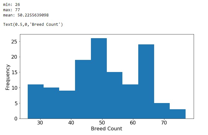
As you can very well see we have a varied distribution of images into different dog classes. Most of the classes have around 50 samples but some are at the extreme lower ends too. There is an imbalance of training data available for different classes.
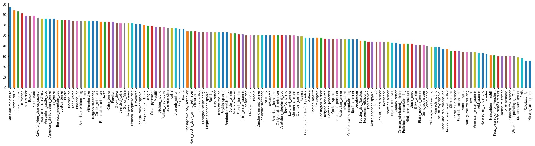 PS. (You may need to open the image in a separate tab for a clearer view)
It becomes clear as we dive into this further, the number of training images for a specific dog breed range from as low as 26 to 77 images per class. This can cause the model to overtrain the classes with large data. But since We don't have a large difference from the mean, it may be acceptable. But definitely, countering this imbalance would help increase the model accuracy by some points. This can be taken up later as a separate exercise to make the model perfect.
Step 1: Detecting Humans:
For detecting human faces, we will leverage OpenCV's implementation of Haar feature-based cascade classifiers. OpenCV provides pre-trained face detectors which are stored as an XML file in the haarcascades folder in our project repo.
#extract pre-trained face detector
face_cascade = cv2.CascadeClassifier('haarcascades/haarcascade_frontalface_alt.xml')
#load color (BGR) image
img = cv2.imread(human_files[3])
# convert BGR image to grayscale
gray = cv2.cvtColor(img, cv2.COLOR_BGR2GRAY)
#find faces in image
faces = face_cascade.detectMultiScale(gray)
#print number of faces detected in the image
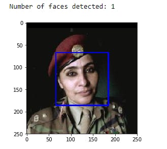
print('Number of faces detected:', len(faces))
#get bounding box for each detected face
for (x,y,w,h) in faces:
#add bounding box to color image
cv2.rectangle(img,(x,y),(x+w,y+h),(255,0,0),2)
#convert BGR image to RGB for plotting
cv_rgb = cv2.cvtColor(img, cv2.COLOR_BGR2RGB)
#display the image, along with bounding box
plt.imshow(cv_rgb)
plt.show()
Sample output:
Step 2: Detecting Dogs:
Now that we have our human face detector in place, moving on to the dog face detector. For this task, we will use the ResNet-50 pre-trained model. This model is trained on a very large, general ImageNet. This is a very popular dataset used for image classification tasks.
def ResNet50_predict_labels(img_path):
    # returns prediction vector for image located at img_path
    img = preprocess_input(path_to_tensor(img_path))
    return np.argmax(ResNet50_model.predict(img))

#Dog detector method
#returns "True" if a dog is detected in the image stored at img_path
def dog_detector(img_path):
    prediction = ResNet50_predict_labels(img_path)
    return ((prediction <= 268) & (prediction >= 151))
Modelling
Pre-processing: For pre-processing of the given data we first use greyscale images to train our model, this is standard practice. Apart from that, we rescale the images by dividing every pixel in every image by 255. This is done to normalize the values on which the model is trained. All the values in the pixel matrix now lie in the range of 0 to 1. In this way the numbers become small and computation becomes easier and faster.
Now let's get to the fun stuff!
Step 3: Create a CNN model from scratch
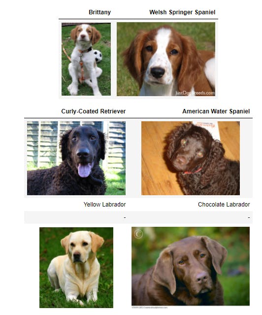
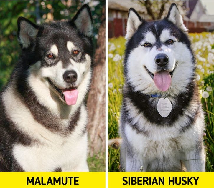
Now that we have created the methods to identify the dog and human faces from input images, we can start working on our model. As you can observe from the image below, it is difficult to identify dog breeds with 100% accuracy even for us humans! This is one of many examples of dog breeds that look almost identical.
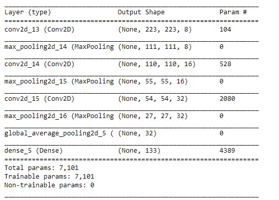
In order to train a model to do the same, we would require a complex architecture that is able to pick up discernable features from the image. For this use case, I decided to go with convolution layers. For dimensionality reduction, I also introduced max-pooling layers. Apart from these layers, I added the final output fully connected layer. Our CNN model looks something like this -
model = Sequential()
model.add(Conv2D(filters=8, kernel_size=2, activation='relu', input_shape=(224, 224, 3)))#init conv layer
model.add(MaxPooling2D(pool_size=2))
model.add(Conv2D(filters=16, kernel_size=2, activation='relu'))
model.add(MaxPooling2D(pool_size=2))
model.add(Conv2D(filters=32, kernel_size=2, activation='relu'))
model.add(MaxPooling2D(pool_size=2))
model.add(GlobalAveragePooling2D())
model.add(Dense(133, activation='softmax')) #output fully connected layer


model.summary()
Training the model:
###TODO: specify the number of epochs that you would like to use to train the model.
epochs = 8
checkpointer = ModelCheckpoint(filepath='saved_models/weights.best.from_scratch.hdf5',
                               verbose=1, save_best_only=True)
model.fit(train_tensors, train_targets,
          validation_data=(valid_tensors, valid_targets),
          epochs=epochs, batch_size=20, callbacks=[checkpointer], verbose=1)
 Evaluating the model:
#get index of predicted dog breed for each image in test set
dog_breed_predictions = [np.argmax(model.predict(np.expand_dims(tensor, axis=0))) for tensor in test_tensors]

#report test accuracy
test_accuracy = 100*np.sum(np.array(dog_breed_predictions)==np.argmax(test_targets, axis=1))/len(dog_breed_predictions)
print('Test accuracy: %.4f%%' % test_accuracy)
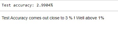
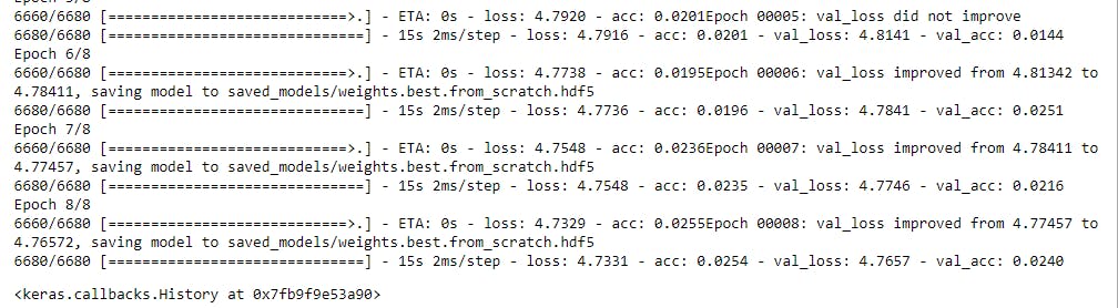
So for our scratch CNN model, test accuracy comes out to be around 3% which is not bad considering we just trained it for 8 epochs. But still, we need an accuracy above 60% for our web app and algorithm to at least be somewhat reliable. We'll do this by implementing transfer learning.
Hyper Parameter Tuning
Step 4: Create a CNN classifier using Transfer Learning
To reduce the training time without sacrificing accuracy we'll train our CNN using transfer learning. We have already discussed about transfer learning in the Overview section so let's just look at how to implement it using python.
Here we will use something known as bottleneck features. In transfer learning in neural networks, we basically remove the last fully connected layer of an existing (pre-trained) model and plug-in our layers there. These layers that we use from the pre-trained model are called bottleneck features. Here, we will be using the ResNet-50 model to extract bottleneck features.
bottleneck_features = np.load('bottleneck_features/DogResnet50Data.npz')
train_Resnet50 = bottleneck_features['train']
valid_Resnet50 = bottleneck_features['valid']
test_Resnet50 = bottleneck_features['test']
#Transfer model architecture
transfer_model = Sequential()
transfer_model.add(GlobalAveragePooling2D(input_shape = train_Resnet50.shape[1:]))
transfer_model.add(Dense(133, activation='softmax'))
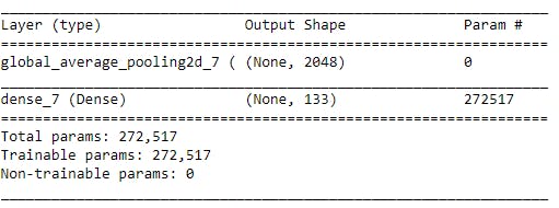
transfer_model.summary()
Training the transfer_model:
#Compile
transfer_model.compile(loss='categorical_crossentropy', optimizer='rmsprop', metrics=['accuracy'])
#Train
checkpointer = ModelCheckpoint(filepath='saved_models/weights.best.Resnet50.hdf5',
verbose=1, save_best_only=True)
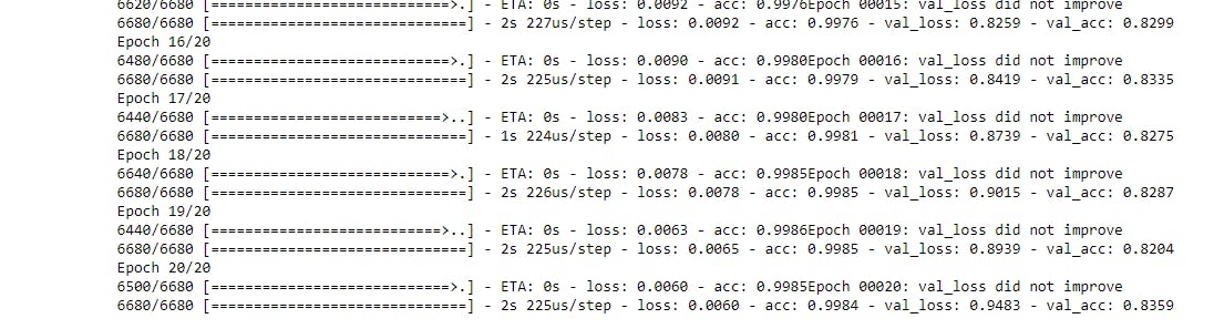
transfer_model.fit(train_Resnet50, train_targets,
validation_data=(valid_Resnet50, valid_targets),
epochs=20, batch_size=20, callbacks=[checkpointer], verbose=1)
transfer_model.load_weights('saved_models/weights.best.Resnet50.hdf5')
transfer_model.save('saved_models/Resnet50_transfer.h5')
Model Evaluation:
#Calculating the classification accuracy on the test dataset.
# get index of predicted dog breed for each image in test set
Resnet50_predictions = [np.argmax(transfer_model.predict(np.expand_dims(feature, axis=0))) for feature in test_Resnet50]
# report test accuracy
test_accuracy = 100*np.sum(np.array(Resnet50_predictions)==np.argmax(test_targets, axis=1))/len(Resnet50_predictions)
print('Test accuracy: %.4f%%' % test_accuracy)

As you can see, using transfer learning, our model has achieved a test accuracy score of 83%. This score can be further improved by training the model on more data or using a different model for transfer learning.
Step 5: Develop the predictor method to classify input images
If you have been paying attention to the code snippets, in step 4 we had saved the best model as an h5 file. Now for inference, we can create a function that uses this trained model to classify the input images into dog breeds.
from IPython.core.display import Image, display
def dog_breed_predictor(img_uri):
bottleneck_feature=extract_Resnet50(path_to_tensor(img_uri))
predicted_vector = transfer_model.predict(bottleneck_feature)
return dog_names[np.argmax(predicted_vector)]
#predictor method to be called for inference
def predictor(img):
display(Image(img, width=350, height=350))
breed=dog_breed_predictor(img).split('.')[-1]
#check for human face
if face_detector(img):
print("This is not a dog! It's a human which looks like:")
return breed
elif dog_detector(img):
print("Dog face detected. Breed is:")
return breed
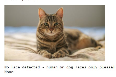
else:
print("No face detected - human or dog faces only please!")
Step 6: Test your method
I have added some test images to the git repo (refer appendix) to test our predictor method. Feel free to test this method on a variety of images.
for i in range(1,7):
    print(predictor("test-img{}.jpg".format(i)))


Results
The Transfer model achieves a test accuracy of 83.5%. Using transfer learning, training time is reduced significantly without an accuracy trade-off. This is a good result for the time it took to train the model. This model can be leveraged to provide classification results reliably.
Conclusion
At the start we set out to build a model to classify dog breeds with an accuracy of atleast 60%. Our scratch CNN model had an accuracy of 3%. Then, on implementing transfer learning we say the accuracy rose to 83% which is a huge improvement!
Indeed with some improvements summarized in the next section, the test accuracy can be improved further. But in conclusion, this model is reliable enough to be deployed as a web app.
Improvements
- The next steps include creating a flask app to use this model to predict dog breeds in real-time.
- The model accuracy can be further improved by using more images for training, trying out some other approaches, or trying out a different pre-trained model.
- The model can be improved by using image augmentation, this would increase the training data. Apart from this tuning the parameters for CNN can also help in achieving a higher accuracy.
If you'd like to play around with the code, the links for the github repo are given in the appendix section. You can also read more about the different concepts used here by taking a look at the references.